There is a lot of discussion of how economic slack is fast disappearing, and I expect a lot of push on this view, given continued rapid growth in GDP as reported in today’s second release for 2014Q3. This view seems counter to (1) the CBO estimate of potential GDP and (2) the slow pace of inflation. My suggestion is that there remains a substantial amount of slack out there.

In Figure 1, I plot log GDP as reported in today’s release, and potential GDP as estimated by the CBO in its August report.

Figure 1: Log GDP (blue), potential GDP as estimated by CBO (gray), and an estimate of potential GDP estimated by use of a modified Ball-Mankiw (2002) method (red). NBER defined recession dates shaded gray. Source: BEA 2014Q3 2nd release, CBO, An Update to the Budget and Economic Outlook (August 2014), NBER, and author’s calculations.

According to the CBO’s estimate of potential (if readers find my repetitive use of the adjective “estimate” tiresome, blame reader Tom), the current (estimated) output gap is -3.5% (in log terms). As I have discussed, there are a variety of other methods than the CBO’s (which is essentially a production function approach), including statistical detrending methods such as the Hodrick-Prescott filter (see [1] [2] [3])

I am going to use economics to infer the output gap and hence the level of potential GDP, i.e., exploiting the expectations-augmented Phillips curve. This means I am appealing to the following data.

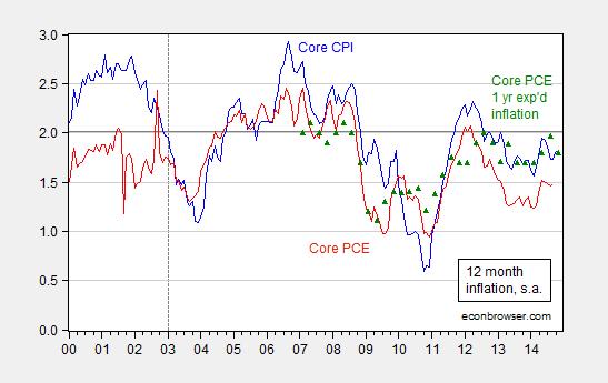
Figure 2: Year-on-year core CPI inflation (blue), core personal consumption expenditures (PCE) deflator (red), and expected one year PCE inflation over the next year (green triangles). Source: BLS, BEA via FRED, Survey of Professional Forecasters.

The methodology is basically that forwarded by Ball and Mankiw (JEP, 2002), which involves inverting a simple expectations-augment Phillips Curve (without supply shocks, but allowing for random shocks), and assuming adaptive expectations (consistent with the accelerationist hypothesis).

πt = πet – a(Ut-U*t) + vt
Δ πt = a U*t – a Ut + vt
U*t + vt/a = Ut + Δ πt/a 
Notice that NAIRU plus a random error is equal to actual unemployment plus the change in inflation divided by a.
This suggests that NAIRU can be estimated by filtering the object on the right side of the last equation.
I follow the same procedure, replacing NAIRU with potential GDP, and using core personal consumption expenditure deflator inflation (q/q at annualized rates).
y*t – vt/a = yt – Δ πt/a

I estimate the analogous a parameter over the 1967Q1-2002Q4 period (so I’m assuming the accelerationist model holds over this sample); the estimate I obtain is approximately 0.08. (See this post for an earlier implementation.) I further assume that expected inflation equals 2% over the 2003Q1-2014Q3 period — which is pretty close to the average 1-year-ahead CPI inflation rate reported by the Survey of Professional Forecasters over this period. In other words, I am assuming that inflation expectations are now well-anchored.

I then HP filter the variable (yt – Δ πt/a) using the default smoothing parameter for quarterly data suggested by Hodrick and Prescott, to obtain an estimate of potential GDP shown in Figure 1 (red line).

What is interesting is not the exact path of estimated potential GDP, but rather that — using this method — the (estimated) output gap as of 2014Q3 is -6.0% (log terms). That is not to say this estimate is “better” than the others; just that there are various indicators of slack — some of which indicate more slack than others –, and it makes sense to appeal to several measures in these uncertain times, as argued by Elias, Irvin, and Jordà.