About twenty years ago, while visiting the Research Department of the IMF, Guy Meredith poked his head in my office and wondered aloud whether interest differentials could reliably predict (in the right direction) subsequent exchange rate changes at horizons of three to five years. The resulting paper led in turn to production of this graph:

Figure 1: Panel beta coefficients at different horizons. Notes: up to 12 months, panel estimates for 6 currencies against US$, euro deposit rates, 1980Q1-2000Q4; 3-year results are zero-coupon yields, 1976Q1-1999Q2; 5 and 10 years, constant yields to maturity, 1980Q1-2000Q4 and 1983Q1-2000Q4 (last observation corresponds to exchange rate data). Source: Chinn (2006).

The Fama regression is:
(1)   st+k – st = α + β(itk-itk*) + εt+k

Where s is the log exchange rate defined as home currency units per foreign currency unit (e.g., USD per pound for Americans); itk is the interest rate of maturity remaining k, and * denotes foreign (e.g., UK); and ε is an error term.

Properly speaking, β=1 is the joint hypothesis of uncovered interest parity and rational expectations (so that forecasting errors of the exchange rate are true innovations), but “Long Horizon Unbiasedness” wasn’t as catchy a title as “Long Horizon UIP”.

What do the data look like? Here are graphs for UK and euro area (vs. US):

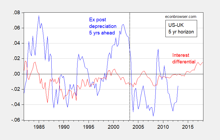
Figure 2: Five year ex post annualized depreciation of dollar/pound exchange rate (higher values denote depreciation of USD) (blue), five year US-UK government bond interest differential (red). The exchange rate depreciation for 2003Q2 pertains the ex post exchange rate change from 2003Q2 to 2008Q2. Dashed line pertains to last exchange rate observation of pre-crisis sample. All data monthly average of daily data for last month of each quarter. Both interest rates constant maturity. Source: Federal Reserve via FRED, Bank of England, and author’s calculations.

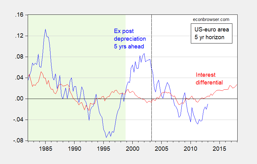
Figure 3: Five year ex post annualized depreciation of dollar/euro exchange rate (higher values denote depreciation of USD) (blue), five year US-Germany government bond interest differential (red). The exchange rate depreciation for 2003Q2 pertains to the ex post exchange rate change from 2003Q2 to 2008Q2. Dashed line pertains to last exchange rate observation of pre-crisis sample. Light green denotes pre-euro area (synthetic euro data used). All data monthly average of daily data for last month of each quarter. Both interest rates constant maturity. Source: Federal Reserve via FRED, ECB, and author’s calculations.

Here are the results I obtained, for the period 1982Q1-2013Q1 (for the interest rates; the exchange rate depreciations are then 1987Q1-2018Q1). I report estimates for β for subsamples before the crisis (1982Q1-2003Q2) and after the crisis (2003Q3-2013Q1). (For an earlier re-assessment, see here; the ending depreciation is 2011Q4, so the last interest rate observation used is 2006Q4).

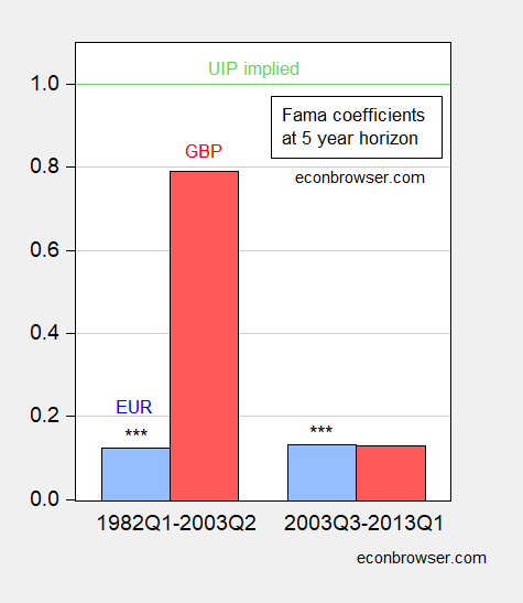
Figure 4: β estimate from equation (1), where t+k is t+20 where frequency is quarterly. Sample period pertains to interest rate data. *** denotes significant difference from unbiasedness value of 1 using HAC robust standard errors. Early euro β estimate incorporates synthetic euro data; late euro β is from a regression including Spain-Germany 10 year spread. Source: author’s calculations.

The euro coefficient in the latter period is negative in the basic specification. UIP relies on default rates that are equal across debt instruments. During the 2010-13 period, sovereign rates for GIIPS countries included some default risk, which would have influenced the exchange rate (recall, we are using German bund yields). Hence, I included the Spanish-German ten year spread to account for this factor, and the reported β estimate reflects this modification.

It would be nice to report that either there were big changes — or no big changes — in long horizon UIP (more correctly long horizon unbiasedness). However, the results are better characterized as ambiguous. For the dollar-pound rate, the point estimate changes substantially; however the degree of imprecision particularly in the latter period means that one can’t reject the null of unity in either case. In addition, one could not reject the null hypothesis the slope coefficient was the same across both periods (although one could reject the null that the constant was the same across both samples). This could merely reflect the low power of the test, when there are relatively few independent observations (recall there are only two completely non-overlapping five year periods in the later subsample, for instance — this is the drawback of using long horizon data).

For the euro, we are hampered by the short sample period (the euro only comes into existence in 1999) and the complications associated with the euro area crisis. I use synthetic euro data to extend the sample, and incorporate the spread variable. A comparison then suggests little change, with the coefficient positive, but significantly different from 1.

In sum, it seems the dollar-pound results are more representative, and indicate continued long horizon UIP. Of course, this is less surprising, in a way, in the latter period given the discussion of the fact that at the short horizon, interest rate point in the right direction for subsequent exchange rate changes, as documented by Bussiere, Chinn, Ferrara and Heipertz (discussed in this post, and this post.)