The New Enhanced Bond Rotation Strategy With Adaptive Bond Allocation
On November 2013 I published an article on the Bond Rotation Strategy (BRS) Now, 15 months later, I am presenting an important update for this strategy. Even though the old strategy has done well (see charts here), I think it is very important to constantly validate and improve any investment strategy. Markets change, ETFs change, even we ourselves grow and learn. I am still improving my knowledge and striving to pass on that knowledge.
In November 2014 I presented the Universal Investment Strategy which was based on a variable allocation of the SPY-TLT ETFs.
This new concept of an ETF rotation with variable allocation is very versatile and can be used on all types of strategies. For the BRS strategy, this new way to calculate allocations results in a considerably improved Sharpe (Return/Risk) ratio of the strategy.
Here is the ETF selection for the BRS
| Old ETF selection | New ETF selection |
| CWB - SPDR Barclays Convertible Bond | CWB - SPDR Barclays Convertible Bond |
| JNK - SPDR High-Yield Junk Bond (4-7yr) | JNK - SPDR High-Yield Junk Bond (4-7yr) |
| TLH - iShares 10-Year Treasury (9-11yr) | TLT - iShares Long-Term Trsry (15-18yr) |
| PCY - PowerShares Emerging Mkts Bond (7-9yr) | |
| AGG - iShares Core Total US Bond (4-5yr) | not necessary anymore |
| BOND - PIMCO Total Return ETF | not necessary anymore |
| SHY - Barclays Low Duration Treasury (2-yr) | not necessary anymore. The total allocation can go automatically below 100% |
An advantage of the adaptive allocation is that we can work with fewer ETFs. We do not need the total return ETFs (AGG, BOND) anymore. The old BRS used these ETFs to achieve a blended way of investing in treasuries and corporate bond ETFs. This was needed because normal switching strategies don’t take into account cross-correlation between ETFs. I had to add total return ETFs so that the strategy ‘knew’ about the possible Sharpe ratio of a blended ETF.
The new strategy, however, does calculate cross-correlations and it will allocate automatically to the top ETFs, so that the Sharpe ratio is maximized.
Cross-correlation is extremely important. If for example the stock market is doing well, then a normal ranking ETF strategy would probably invest in the two highly correlated corporate bonds: JNK and CWB. However a combination of CWB with a negatively correlated treasury TLT would probably have the better Sharpe ratio because of the inverse correlation of the two ETFs. This would reduce volatility and this would result in a higher Sharpe ratio for this ETF pair.
For the selection of the 4 ETFs, it was very important to have uncorrelated bonds, so that we would have successful ETF combinations for any kind of market.
| ETF | Average correlation to the stock market (SPY) |
| CWB - SPDR Barclays Convertible Bond | 0.8 |
| JNK - SPDR High-Yield Junk Bond (4-7yr) | 0.7 |
| PCY - PowerShares Emerging Mkts Bond (7-9yr) | 0.25 |
| TLT- iShares Long-Term Trsry (15-18yr) | -0.5 (-0.75 during market corrections) |
The new PCY Emerging market bond ETF is an interesting addition with low correlation to the other ETFs. From a correlation point of view, it sits halfway between stocks and treasuries, and it gives the strategy some additional global diversification.
To calculate the strategy we use our QuantTrader software. As this is a top 2 ETF strategy, the algorithm calculates the maximum Sharpe allocation for all 6 possible ETF pairs. We could run allocations from 0% to 100% for each ETF, but for the bond rotation it is better to limit the allocations from a 40% minimum allocation to a maximum of 60%. If we allow bigger variations the risk increases because there would be times where we are invested up to 100% in one single ETF. The return would also increase, but the Sharpe ratio would be lower than with this 40%-60% allocation.
One way to further improve risk adjusted returns would be to always invest in all 4 ETFs with adaptive allocation. The algorithm would loop through all allocations like 10%-30%-20%-40% and calculate the max Sharpe allocation considering the cross correlation of all 4 ETFs. For bigger investments, this would be the best solution with the highest Sharpe ratio and a very low volatility of only 5%. It is also good because the ETF risk is spread among 4 ETFs rather than 2 ETFs. However for the private investor an investment in the best 2 ETFs is absolutely sufficient.
The new BRS strategy shares the same tweaked Sharpe formula with the UIS strategy. Normally the Sharpe ratio is calculated by Sharpe=rd/sd with rd=mean daily return and sd= standard deviation of daily returns. I don’t use the risk free rate, as I only use the Sharpe ratio to do the ranking. My algorithm uses the modified Sharpe formula Sharpe=rd/(sd^f) with f=volatility factor. The f factor allows me to change the importance of volatility. If f=0, then sd^0=1 and the ranking algorithm will choose the composition with the highest performance without considering volatility. If f=1, then I have the normal Sharpe formula. Using values of f>1, I rather want to find ETF combinations with low volatility. With high f values, the algorithm becomes a “minimum variance” or “minimum volatility” algorithm.
Here is a comparison between different ways to execute the BRS:
Comparison of different BRS strategies (5 year)
| Strategy | 5 year CAGR | Sharpe ratio | Max drawdown | |
| 1 | Old BRS strategy (top 1 ETFs) | 11% annual return | 1.13 | -12.2% |
| 2 | Old BRS strategy (top 2 ETFs) | 12.5% annual return | 1.44 | -9.3% |
| 3 | New BRS strategy (2 ETFs) | 17% annual return | 2.25 | -6.5% |
| 4 | New BRS strategy (4 ETFs) | 13% annual return | 2.45 | -6.6% |
| 5 | AGG (benchmark) | 4.18% annual return | 1.25 | -5.1% |
| 6 | SPY (benchmark) | 15.9% annual return | 1.01 | -18.6% |
N.B. - no. 3 is the strategy used by Logical-Invest
The max drawdown coincides with the end of QE announcement in 2013. Bond strategy drawdowns are mostly driven by Fed announcements, but they are about 3x smaller than SPY drawdowns.
Here is a screenshot of the 5 year backtest of the new BRS with QuantTrader
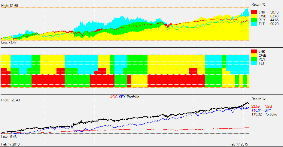
The middle graph shows the allocation of the ETFs and the lower graph shows the strategy compared to two benchmarks: AGG total return bond ETF and SPY S&P 500 ETF.
Due to the limited history of the corporate bond ETF CWB, which exists only since 2009, this backtest is quite short. However, using mutual fund proxies we can backtest the strategy using a longer historical period.
There is a plenitude of different proxies using mutual funds, but none is a 100% match. In particular, emerging market bonds are only available in recent times. Still they add unique diversity.
Long-term backtests are interesting, but personally I don’t think that you need to look back longer than 10 years. Markets and ETFs evolve so quickly that history that extends back for more than 5 years is not really useful in fine-tuning a strategy which has to successfully trade in current market conditions and whose only goal is to predict the next 20 trading days.
So take the results below with a grain of salt. They show that the fundamental principle of the strategy works even before 2008. It does perform even better after 2008 due to increased momentum of stock and bond markets after the 2008 correction.
The most important lesson learned from this longer term backtest is that you don’t need to be afraid of big market corrections. Such corrections are even good for strategies with variable allocation, because you can make double the gains: once using defensive Treasuries during the downgoing market, and then a second time when the markets go up again.
Mutual fund proxies used for the longer term backtest
| ETF | Proxy |
| TLT - iShares Barclays Long-Term Trsry (15-18yr) | VUSTX - Vanguard Long-Term Treasury Inv |
| JNK - SPDR Barcap High-Yield Junk Bond (4-7yr) | PRHYX - T. Rowe Price High-Yield |
| PCY - PowerShares Emerging Mkts Bond (7-9yr) | RPIBX - T. Rowe Price International Bond |
| CWB - SPDR Barclays Convertible Bond | VCVSX - Vanguard Convertible Securities Inv |
| Benchmark: AGG - iShares Core Total US Bond (4-5yr) | Benchmark: VBMFX - Vanguard Total Bond Market Index Inv |
Here is a screenshot of the 13 year backtest of the mutual fund BRS with QuantTrader
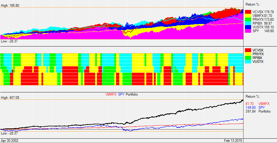
The charts show that the strategy worked well since 2002. CAGR is 13.2% and Sharpe is 2.02. The max drawdown was 12.5% in 2008. However one last important question for the future is how the strategy will handle rising rates?
I think that the BRS should still do quite well in a rising rate environment, because of the two corporate bonds CWB and JNK. Long duration 15-18 year Treasury bonds (TLT) will be affected most by rising rates. But even here I would set a question mark. With Treasury yields near zero in Europe, these US long term bonds are still extremely attractive. Convertible corporate bonds or high yield bonds with short duration and a high coupon are even more attractive and should do quite well in a rising rate environment. Emerging-markets bonds like PCY are quite susceptible to global sentiment, but they should be less affected by rising rates also because of their lower 9 year duration.
All I know is, the banks and Federal Reserve have been constantly wrong about their predictions on rising rates for five years, so be skeptical of any rate predictions. Better let algorithms decide how to change bond allocations.
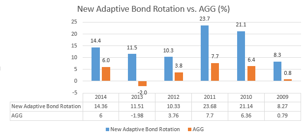
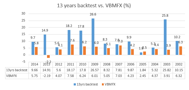
Here is the Annual Performance in comparison: